ISSN 2307–3489 (Print), ІSSN 2307–6666 (Online)

Наука та прогрес транспорту. Вісник Дніпропетровського
національного університету залізничного транспорту, 2018, № 6 (78)

МОДЕЛЮВАННЯ ЗАДАЧ ТРАНСПОРТУ ТА ЕКОНОМІКИ

Introduction

One of the main requirements for routing algorithms is their rapid matching to an optimal solution, dictated by the need for their protocol realization in real time in the conditions of continuous change in the characteristics of network traffic, topology and load of computer networks used in the rail transport. Classic algorithms for finding the shortest path on the graph used in modern routing protocols cannot do this. One of the approaches to solving routing problems in computer networks is the use of neural network technology [8, 15–16]. For example, in [12] it is shown that with the help of a neural network (NN) it is possible to find a solution, close to the optimal, to the travelling salesman problem and to find the shortest path on the graph. In [3] for solving routing problems there is studied the possibility of applying the following neural networks: Multi Layer Perceptron; RBF network; Hopfield network. It is established that the most promising means for solving the routing problem are the direct distribution neural network and the Hopfield network, which are capable of operating under conditions of dynamic change in the topology of the computer network and the characteristics of the data transmission channels [1–2]. In particular, when using the Hopfield network, additional research is required on the transfer functions of the neurons and on the energy of the neural network [18]. In [7], it was discovered that the Hopfield network finds a satisfactory route that differs from the optimal one by 7-8% in ave-rage (in the case of more than 15 seats). The possibility of using the Hopfield network to find the shortest path on the route graph in the computer network of railway transport is analysed [5–6]. In [3], the use of the direct distribution neural network created in MatLAB for the purpose of determining the route in a computer network of five nodes was investigated. But the integrated computer network of rail transport consists of a much larger number of nodes, which requires additional research. In particular, [20] proposed an intellectual control subsystem with the use of network technology, [17] – a subsystem of prediction based on a neural fuzzy network.

Purpose

To develop a methodology for determining the optimal route in the unified computer network based on the created software model «MLP34-2-410-34» using the TensorFlow framework.

Methodology

A combined computer network that works on different technologies can be represented as an unoriented graph G (V, W), where V is the set of graph vertices, the number of which is N, with each vertex modelling a node (router) of the computer network; W is the set of graph edges, the number of which is M. Each graph edge is assigned with a certain weight corresponding to the bandwidth (the maximum amount of data transmitted by the network per unit time):

, (1)

where – bandwidth of the communication channel between the i-th and j-th network nodes, Mbps.

To solve the routing problem, it is necessary to find the optimal path between the two routers assigned to the unified computer network. As an example, we will consider a hypothetical computer network whose structure is shown in Fig. 1

Let us introduce the array:

, (2)

where – availability of traffic transmitted within the network between the i-th and j-th vertices. As a limit , i.e. the variable takes value 1, if the traffic flows through the channel (i, j); otherwise – 0.

As the criterion of optimality, the following expression is supported:

, (3)

where , which guarantees the search for a path with the maximum bandwidth.

If there is no connection between the nodes of the unified computer network, then c_ij = c_ji = 0 (hence, ).

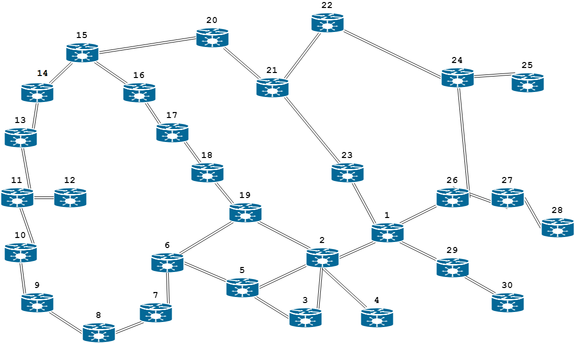
Fig. 1. Graph of router connections of unified computer network

Findings

Neural network as the main mathematical tool for solving the problem. In the unified computer network there are 30 routers and 34 communication channels. As an example, let us consider the solution to the problem of determining the optimal route between the nodes «12» and «1». Generally between the indicated nodes there are 14 unique paths.

Path 1: [12, 11, 13, 14, 15, 20, 21, 23, 1];
path 2: [12, 11, 10, 9, 8, 7, 6, 19, 2, 1];
path 3: [12, 11, 10, 9, 8, 7, 6, 5, 2, 1];
path 4: [12, 11, 10, 9, 8, 7, 6, 5, 3, 2, 1];
path 5: [12, 11, 13, 14, 15, 16, 17, 18, 19, 2, 1];
path 6: [12, 11, 13, 14, 15, 20, 21, 22, 24, 26, 1];
path 7: [12, 11, 13, 14, 15, 16, 17, 18, 19, 6, 5, 2, 1];
path 8: [12, 11, 13, 14, 15, 16, 17, 18, 19, 6, 5, 3, 2, 1];
path 9: [12, 11, 10, 9, 8, 7, 6, 19, 18, 17, 16, 15, 20, 21, 23, 1];
path 10: [12, 11, 10, 9, 8, 7, 6, 19, 18, 17, 16, 15, 20, 21, 22, 24, 26, 1];

path 11: [12, 11, 10, 9, 8, 7, 6, 5, 2, 19, 18, 17, 16, 15, 20, 21, 23, 1];
path 12: [12, 11, 10, 9, 8, 7, 6, 5, 3, 2, 19, 18, 17, 16, 15, 20, 21, 23, 1];
path 13: [12, 11, 10, 9, 8, 7, 6, 5, 2, 19, 18, 17, 16, 15, 20, 21, 22, 24, 26, 1];
path 14: [12, 11, 10, 9, 8, 7, 6, 5, 3, 2, 19, 18, 17, 16, 15, 20, 21, 22, 24, 26, 1].

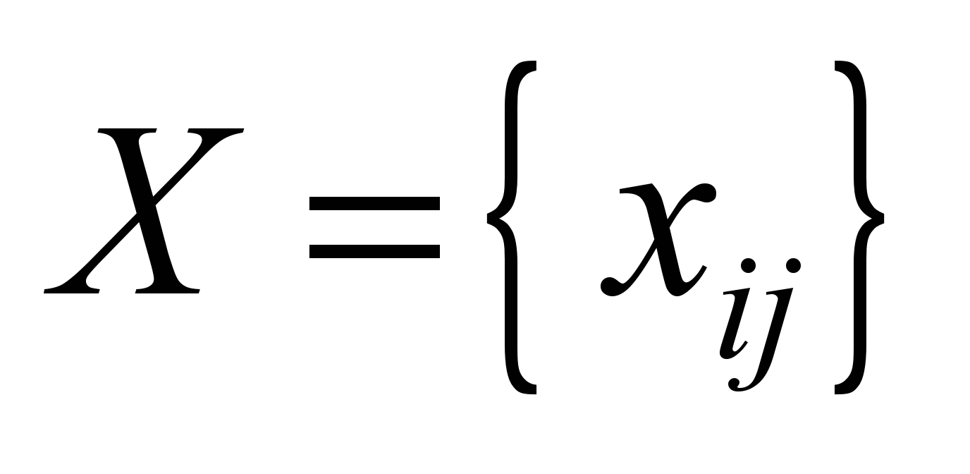
To solve the routing problem, we used the NN, whose structure is shown in Fig. 2. To the NN input, there is applied a vector of bandwidth of the channels of the unified computer network X, which characterizes its current state X = {xi}, where i = 1, ..., m (m = 34). For example, for NN, when using the train sample of 1,400 examples, the number of required neurons in the hidden layer is estimated as follows:

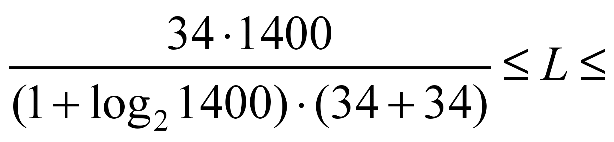
Hence, .

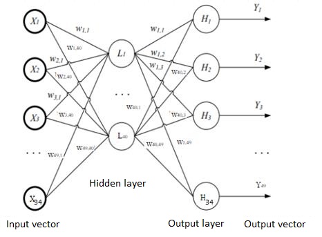
Fig. 2. Structure of multilayer NN

Sample preparation (preparatory stage). Formation of the sample is carried out according to the fixed structure of the unified computer network (see Fig. 1). The input vector X is constructed by randomly generating channel bandwidth values , while these values are formed by a uniform distribution onto the segments [100; 100,000,000]. The response vector Y is generated by calculating the optimal path according to the Dijkstra algorithm using the Python language of the Networkx library (open source software library used to work with graphs and networks).

The samples are constructed so that each of 14 unique paths is present at the same frequency. The test sample has 700 examples, validation sample has 700 examples, the first train sample has 140 examples (10 examples for each path), the second train sample has 1,400 examples (100 examples for each path), the third training sample – 14,000 examples (1,000 examples for each path), the fourth train sample – 49,000 examples (3,500 examples for each path).

All data is initially normalized to the range from 0 to 1 by the formula:

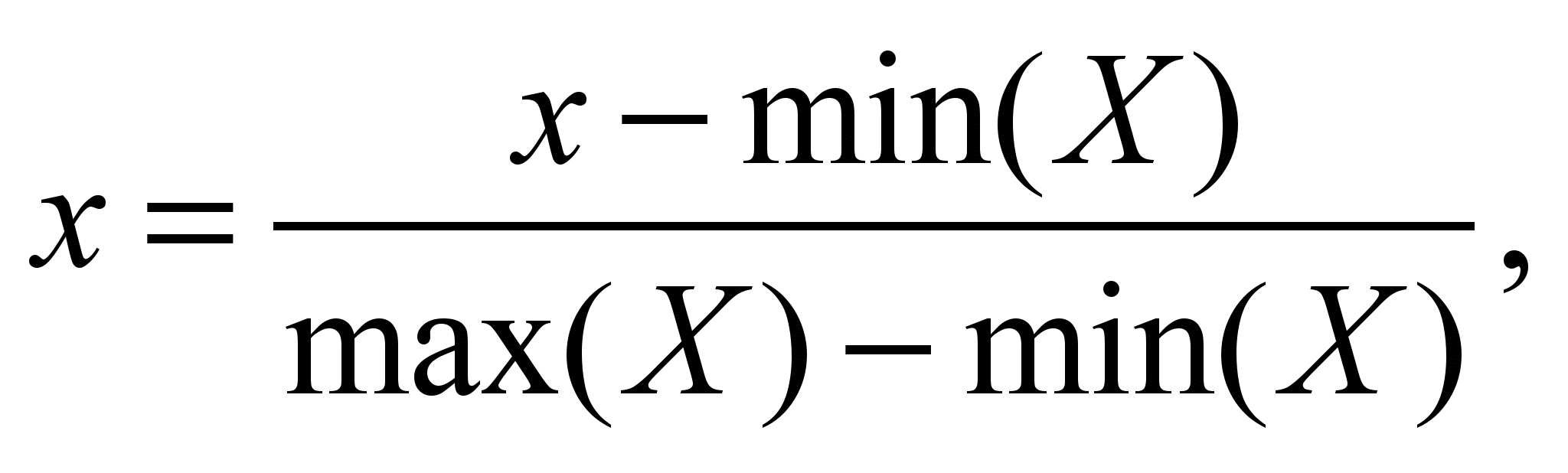
(4)

The structure of the resulting vector is as follows: Y = [y_1,2, y_1,26, y_1,29, y_1,23, y_2,19, y_2,3, y_2,5, y_2,4, y_3,5, y_5,6, y_6,19, y_6,7, y_7,8, y_8,9, y_9,10, y_10,11, y_11,12, y_11,13, y_13,14, y_14,15, y_15,16, y_15,20, y_16,17, y_17,18, y_18,19, y_20,21, y_21,22, y_21,23, y_22,24, y_24,25, y_24,26, y_26,27, y_27,28, y_29,30], where , that corresponds to using or not using the appropriate channel in the route.

Justifying the choice of modelling tools. To solve the routing problem in the unified computer network, the Keras library was selected using TensorFlow and Numpy in the Python programming language [9–11, 13–14, 19].

Keras is an open neural network library in Python language capable of working on top of Deeplearning4, TensorFlow and Theano, designed for quick neural network deep learning experiments.

TensorFlow is an open source software library for machine learning. It is the second-generation GoogleBrain machine learning system released as open source software.

Numpy is an extension of the Python language that supports large, multidimensional arrays and matrices, along with a library of high-level mathematical functions for operations with these arrays.

Python is an interpreted object-oriented high-level programming language with strict dynamic typing. High-level data structures, along with dynamic semantics and dynamic linking, make it attractive for rapid development of applications, as well as a tool for existing components. Python supports modules and module packages, which facilitates modularity and reuse of the code. Python interpreter and standard libraries are available both in compilation and in source form on all major platforms. Python programming language supports several programming paradigms, including: object-oriented; procedural; functional; aspect-oriented.

Structure of MLP 34-2-410-34 software model. MLP 34-2-40-34 software model, created for mo-delling and research, consists of the main module «Main» and the following classes: Generator, MLPModel, NetworkX, Matplotlib, Keras.Model, Metrics, Tensorflow. The main module «Main» provides the menu tasks: 1 – sample generation;
2 – neural network training; 3 – neural network testing. «Generator» performs a sample preparation in two modes: random (calculating the random number of examples for each path, Fig. 3, a); balanced (the same number of examples for each possible path, Fig. 3, b). For example, a sample of 140 examples in balanced mode takes 5 minutes, while in random mode it takes less than one minute.

                                                                                                                             a                                                                                                    b

Fig. 3. Generation of sample:
a –random; b –balanced

«MLPModel» creates a neural network of 34-2-X-34 configuration (where X is the possible number of hidden neurons) and performs the following steps: training; testing; control on the corresponding samples and their normalization.

«NetworkX» (standard class) builds a graph of the computer network (Graph), calculates the existing paths between stations (all_simple_paths), the path between the specified stations according to the Dijkstra algorithm (bidirectional_dijkstra).

«Matplotlib» (standard class) builds a pie chart and histogram to show the ratio of the number of examples for each path.

«Keras.Model» (standard class) performs compilation in accordance with the given configuration of the neural network (compile), represents the standard functions (fit, predict) that are used during the training and testing of the neural network.

«Metrics» performs the calculation of the pro-bability of the optimal and of correct answers.

«TensorFlow» (standard class) is called by the «Keras.Model» class when performing the appropriate calculations.

The overall structure of MLP 34-2-40-34 software model is shown in Fig. 4

In order to be able to unambiguously compare the NN models in two parameters – the probability of optimal responses and the probability of correct responses, we entered the value of the harmonic mean, which is calculated by the following formula:

, (5)

where – probability of optimal responses, – probability of correct responses.

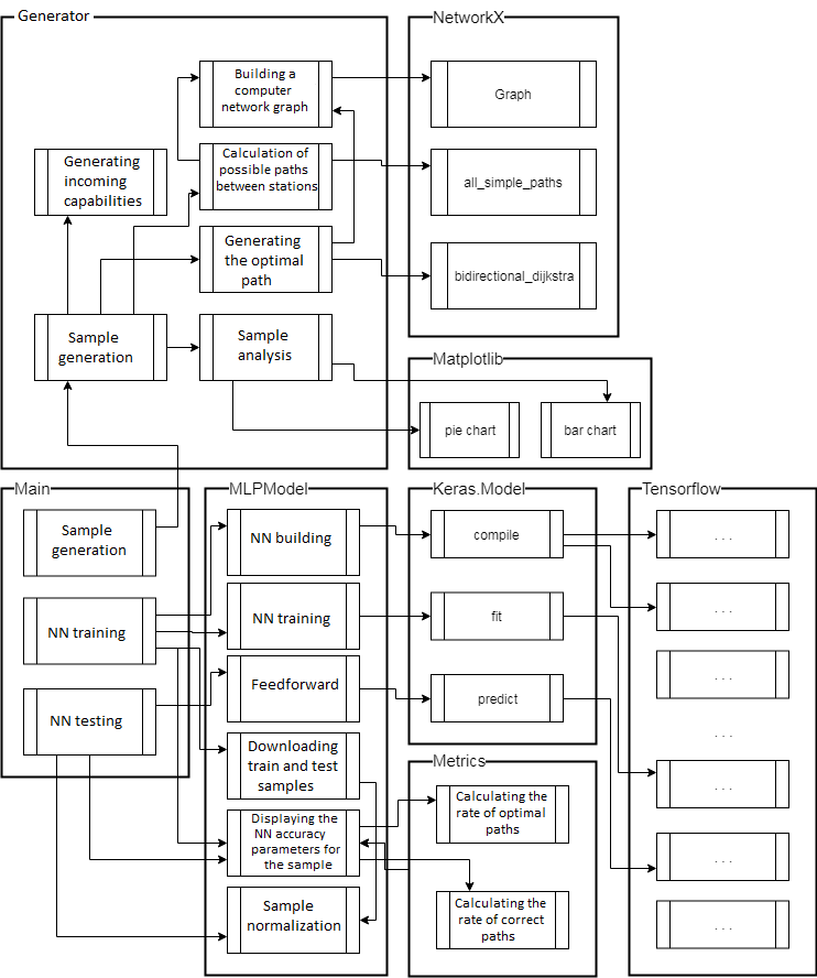
Fig. 4. Structure of MLP 34-2-40-34 software model

Testing MLP34-2-410-34 program. The resulting feature vector of channel entry to the optimal path is as follows: {0,0,0,1,0,0,0, 0,0,0,0,0,0,0,0,0,1,1,1,1,0,1,0,0,0,1,0,1,0,0,0,0,0,0}, which corresponds to the following connection of routers in the network:1–23, 11–12, 11–13, 13–14, 14–15, 15–20, 20–21, 21–23. The resulting path is shown in Fig. 5

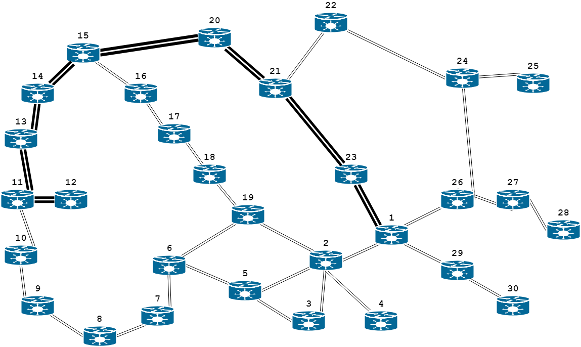
Fig. 5. The resulting optimal path consisting of channels:
12–11, 11–13, 13–14, 14–15, 15–20, 20–21, 21–23, 23–1

Study of the NN training effectiveness for different number of neurons in the hidden layer. The study on the NN model was performed using the stochastic gradient descent algorithm (batch size 64) with Adam optimization (training speed α = 0.001, inertia , RMSprop , ) on 1,400 study examples, over 1,000 epochs for different numbers of hidden neurons: .

The results of the experiment are shown in the Table 1. From the table it is clear that for the train sample the best result of 0.99 is already achieved with 410 neurons in the hidden layer.

Table 1

Study of NN for different number of hidden neurons

Number of hidden neurons		62	410	760	1 110	1 456
Train sample		0.77	0.99	0.99	0.99	0.99
		0.81	0.99	0.99	0.99	0.992
	H	0.79	0.99	0.99	0.99	0.99
Test sample		0.55	0.52	0.51	0.52	0.51
		0.71	0.7	0.69	0.7	0.71
	H	0.62	0.6	0.59	0.6	0.59

The NN training process is illustrated in the objective function-epoch dependency graphs for the train and test samples in Fig. 6-10.

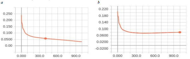
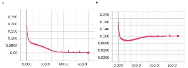
Fig. 6. The 34-2-64-34 NN error-epoch dependency graph on samples:
a – train; b – test

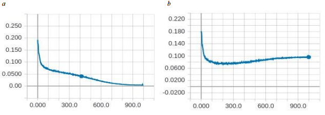
Fig. 7. The 34-2-410-34 NN error-epoch dependency graph on samples:
a – train; b – test

Fig. 8. The 34-2-760-34 NN error-epoch dependency graph on samples:
a – train; b – test

Fig. 9. The 34-2-1110-34 NN error-epoch dependency graph on samples:
a – train; b – test

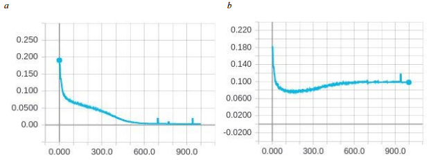
Fig. 10. The 34-2-1456-34 NN error-epoch dependency graph on samples:
a – train; b – test

Figures 6-10 show that all of the proposed NN models feature re-training after the 200^th epoch. Since the NN model of 34-2-410-34 configuration gives the best result for a relatively small number of neurons, it is selected for further research as the most promising one.

Study of the NN training effectiveness for various activation functions and train sample sizes. The efficiency of the 34-2-410-34 NN model is studied for various neuron activation functions in the hidden layer. The output layer has a linear activation function. The training was carried out using the stochastic gradient descent algorithm (batch size 64) with Adam optimization (learning speed α = 0.001, inertia , RMSprop , ) for 1,000 epochs. Experiments were performed for various activation functions in the hidden layer (linear, sigmoid, hyperbolic tangent, Softplus, ReLU, Leaky-ReLU α = 0.1; Table 2) and for different train sample sizes (140, 1,400, 14,000 and 49,000 examples). The results of NN modelling are given in Table 2-4, the NN training process is illustrated in Fig. 11-14.

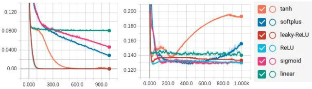
Fig. 11. The MSE error-epoch dependency graph for train and test samples of 140 examples:

The study showed that NN training for Softplus and Sigmoid activation functions did not stop, and it is possible to achieve greater accuracy during further training. In addition, one can see the attri-butes of the NN re-training for Tanh and Softplus activation functions.

Table 2

Study of NN for various activation functions on train sample of 140 examples

Activation function		Linear	Sigmoid	Tanh	Softplus	ReLU	L-ReLU
Train sample		0.28	0.58	1	0.78	1	1
		0.32	0.61	1	0.78	1	1
	H	0.3	0.6	1	0.78	1	1
Test sample		0.07	0.17	0.03	0.1	0.16	0.16
		0.11	0.29	0.05	0.18	0.25	0.28
	H	0.09	0.21	0.04	0.13	0.19	0.2

The table shows that on the small volumes of data the activation functions Sigmoid, ReLU and Leaky-ReLU showed themselves the most successfully on the test sample. The best result of accuracy in training data was shown by the activation functions Tanh, ReLU, Leaky-ReLU, so they can be considered promising for larger sample sizes.

Fig. 12. The MSE error-epoch dependency graph for train and test samples of 1,400 examples.

Table 3

Study of NN for various activation functions on train sample of 1,400 examples

Activation function		Linear	Sigmoid	Tanh	Softplus	ReLU	L-ReLU
Train sample		0.2	0.98	1	0.99	1	1
		0.24	0.99	1	0.99	1	1
	H	0.22	0.98	1	0.99	1	1
Test sample		0.19	0.53	0.06	0.3	0.46	0.46
		0.24	0.7	0.06	0.35	0.61	0.61
	H	0.21	0.6	0.6	0.32	0.53	0.52

The table shows that on the average data volumes, Sigmoid, Tanh, ReLU and Leaky-ReLU activation functions were most successful on the test sample. Except for the linear activation function, all functions have given maximum accuracy on the training data.

Table 4

Study of NN for various activation functions on train sample of 14,000 examples

Activation function		Linear	Sigmoid	Tanh	Softplus	ReLU	L-ReLU
Train sample		0.2	1	0.99	0.99	1	1
		0.24	1	0.99	0.99	1	1
	H	0.22	1	0.99	0.99	1	1
Test sample		0.19	0.66	0.57	0.61	0.76	0.74
		0.24	0.78	0.63	0.67	0.86	0.83
	H	0.21	0.71	0.6	0.64	0.81	0.79

The table shows that on the data volumes bigger than the average, Sigmoid, ReLU and Leaky-ReLU activation functions were most successful on the test sample. Except for the linear activation function, all functions have given maximum accuracy on the training data.

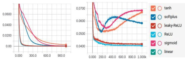
Fig. 13. The MSE error-epoch dependency graph
for train and test samples of 1 14,000 examples

Table 5

Study of NN for various activation functions
on train sample of 49,000 examples

Activation function		Linear	Sigmoid	Tanh	Softplus	ReLU	L-ReLU
Train sample		0.2	1	0.96	1	1	1
		0.24	1	0.96	1	1	1
	H	0.22	1	0.96	1	1	1
Test sample		0.19	0.81	0.8	0.76	0.83	0.85
		0.24	0.86	0.84	0.8	0.9	0.9
	H	0.21	0.83	0.82	0.78	0.86	0.88

Fig. 14. The MSE error-epoch dependency graph for train
and test samples of 49,000 examples

The resulting NN of 34-2-410-34 configuration with the activation function Leaky-ReLU (α = 0.1) in the hidden layer and the linear activation function in the output layer after training with 49,000 examples for 1,000 epochs reached MSE value of 0.0024 on the control sample and in 86% determines the optimal path.

Originality and practical value

The NN of 34-2-410-34 configuration with activation function Leaky-ReLU (α = 0.1) in the hidden layer and with linear function in the output layer was studied. Experiments were conducted for various training optimization algorithms during 100 epochs for the sample size of 49,000 examples. The results of experiments are shown in the table 6, the training process is illustrated in Fig. 15.

According to the results of experiments, it is evident that the NN in the classical gradient descent learns very slowly; the NN in the stochastic gradient descent shows a significant improvement. Adam, AdaMax and Nadam training algorithms showed almost identical results.

Table 6

Study of NN of 34-2-410-34 configuration by different algorithms

Algorithm		BGD	MB SGD	Adam	Adamax	Nadam
Train sample		0	0.09	0.99	0.96	0.99
		0	0.1	1	0.97	0.99
	H	0	0.1	0.99	0.96	0.99
Test sample		0	0.11	0.87	0.85	0.87
		0	0.12	0.92	0.9	0.92
	H	0	0.11	0.89	0.87	0.9

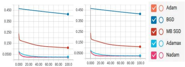
Fig. 15. The MSE error-epoch dependency graph for train
and test samples for different training algorithms

Conclusions

1. The routing problem in the unified computer network is solved based on the developed software model «MLP 34-2-410-34» using the Python language and the TensorfFow framework, which allows generating the samples: train (140, 1 400, 14,000, 49,000 examples); test (700 examples); control (700 examples), as well as modelling the work of the neural network and studying its parameters.

2. Efficiency was studied based on the harmonic mean of the NN of 34-2-X-34 configuration with sigmoid activation function in the hidden layer and linear function in the output layer for different number of hidden neurons: 62; 410; 760; 1 110; 1 456. During NN training we used the modern Adam algorithm for optimizing stochastic gradient descent with recommended hyperparameters: learning speed α = 0.001; inertia ; RMSprop ; . The study showed that the accuracy of the neural network can be reached with 410 hidden neurons, and the further increase does almost nothing to improve the results.

3. Efficiency was studied based on the harmonic mean of the NN of 34-2-410-34 configuration under different activation functions: linear; sigmoid hyperbolic tangen-som; Softplus, ReLU; Leaky-ReLU using the Adam algorithm on train samples of different size (140, 1 400, 14,000, 49 000 examples). The study has shown that the activation functions ReLU and Leaky-ReLU train the most rapidly at all levels of the train sample and less than other activation functions are subject to re-training. The NN of 34-2-410-34 configuration for activation functions Tanh and Softplus can achieve 100% accuracy on the train sample, but these functions are less slowly learned than ReLU and Leaky-ReLU and are strongly subject to re-training with insignificant sizes of the train sample (140, 1,400 and 14,000 examples). When using the sigmoid activation function, the neural network is also retrained, but with a large size of train examples (49,000 examples) it is able to achieve accuracy (83%) close to Leaky-ReLU (88%) or ReLU (86%).

4. Efficiency of the NN of 34-2-410-34 configuration was studied with activation function Leaky-ReLU (α = 0.1) in the hidden layer and with linear function in the output layer. Experiments were conducted by different optimization algorithms (BGD, MB SGD, Adam, Adamax, Nadam) during 100 epochs with the train sample of 49,000 examples. Adam, Adamax, and Nadam algorithms showed almost identical results, with 89, 87, and 90% accuracy, respectively.

LIST OF REFERENCE LINKS

1. Колесніков, К. В. Аналіз результатів дослідження реалізації задачі маршрутизації на основі нейронних мереж та генетичних алгоритмів / К. В. Колесніков, А. Р. Карапетян, В. Ю. Баган // Вісн. Черкас. держ. технол. ун-ту. Серія: Технічні науки. – 2016. – № 1. – C. 28–34.

2. Кутыркин, А. В. Использование нейронной сети Хопфилда для решения оптимизационных задач маршрутизации : метод. указания / А. В. Кутиркин, А. В. Семин. – Москва : Изд-во Моск. гос. ун-та путей сообщения, 2007. – 15 с.

3. Павленко, М. А. Анализ возможностей искусственных нейронных сетей для решения задач однопутевой маршрутизации в ТКС [Electronic resource] // Проблеми телекомунікацій. – 2011. – № 2 (4). – Avai-lable at: http://pt.journal.kh.ua/index/0-139 – Title from the screen. – Accessed : 20.11.2018.

4. Палмер, М. Проектирование и внедрение компьютерных сетей / М. Палмер, Р. Б. Синклер. – Санкт-Петербург : БХВ-Петербург, 2004. – 752 с.

5. Пахомова, В. М. Аналіз методів з природними механізмами визначення оптимального маршруту в комп’ютерній мережі Придніпровської залізниці / В. М. Пахомова, Р. О. Лепеха // Інформ.-керуючі системи на залізн. трансп. – 2014. – № 4. – С. 82–91.

6. Пахомова, В. М. Рішення задачі маршрутизації в комп’ютерній мережі Придніпровської залізниці на основі нейронної моделі Хопфілда / В. М. Пахомова, Ю. О. Федоренко // Інформ.-керуючі системи на залізн. трансп. – 2012. – № 4. – С. 76–84.

7. Реалізація задачі вибору оптимального маршруту нейронною мережею Хопфілда / А. М. Бриндас,
   П. І. Рожак, Н. О. Семинишин, Р. Р. Курка // Наук. вісн. НЛТУ України : зб. наук.-техн. пр. – Львів, 2016. – Вип. 26.1. – C. 357–363.

8. Хайкин, С. Нейронные сети. Полный курс : [пер. с англ.] / С. Хайкин. – 2-е изд., испр. – Москва : Вильямс, 2006. – 1104 с.

9. An open source machine learning framework for everyone [Electronic resource] : [веб-сайт] / TensorFlow. – Електрон. текст. дані. – Available at: https://www.tensorflow.org – Title from the screen. – Accessed : 05.06.2018.

10. A Survey of Artificial Immune System Based Intrusion Detection / Hua Yang, Tao Li, Xinlei Hu, Feng Wang, Yang Zou // The Scientific World Journal. – 2014. – Vol. 2014. – Р. 1–11. doi: 10.1155/2014/156790

11. CiscoTips [Electronic resource] : [веб-сайт]. – Електрон. текст. дані. – Available at: http://ciscotips.ru/ospf – Title from the screen. – Accessed : 20.05.2018.

12. Hopfield, J. J. Neural networks and physical systems with emergent collective computational abilities /
    John J. Hopfield // Proceedings of National Academy of Sciences. – 1982. – Vol. 79. – Іss. 8. – P. 2554-2558. doi: 10.1073/pnas.79.8.2554

13. IBM [Електронний ресурс] : [веб-сайт] / IBM Knowledge Center. – Електрон. текст. дані. – Available at: https://u.to/G-giFA – Title from the screen. – Accessed : 20.05.2018.

14. Keras [Electronic resource] : [веб-сайт]. – Електрон. текст. дані. – Available at: https://keras.io/ – Title from the screen. – Accessed : 05.06.2018.

15. Neural Network Based Near-Optimal Routing Algorihm / Chang Wook Ahn, R. S. Ramakrishna, In Chan Choi, Chung Gu Kang // Neural Information Processing, 2002. ICONIP'02 : Proc. of the 9th Intern. Conf. (18–22 Nov. 2002). – Singapore, 2002. – Vol. 5. – P. 1771–1776. doi: 10.1109/iconip.2002.1198978

16. New algorithm for packet routing in mobile ad-hoc networks / N. S. Kojić, M. B. Zajeganović-Ivančić,
    I. S. Reljin, B. D. Reljin // Journal of Automatic Control. – 2010. – Vol. 20. – Іss. 1. – P. 9–16.
    doi: 10.2298/jac1001009k

17. Pakhomova, V. M. Network Traffic Forcasting in information-telecommunication System of Prydniprovsk Railways Based on Neuro-fuzzy Network // Наука та прогрес транспорту. – 2016. – № 6 (66). – C. 105–114. doi: 10.15802/stp2016/90485

18. Schuler, W. H. A novel hybrid training method for hopfield neural networks applied to routing in communications networks / W. H. Schuler, C. J. A. Bastos-Filho, A. L. I. Oliveira // International Journal of Hybrid Intelligent Systems. – 2009. – Vol. 6. – Іss. 1. – P. 27–39. doi: 10.3233/his-2009-0074

19. Security Lab.ru [Електронний ресурс] : [веб-сайт]. – Електрон. текст. дані. – Режим доступу: https://www.securitylab.ru/news/tags/UDP – Назва з екрана. – Перевірено : 20.05.2018.

20. Zhukovyts’kyy, I. Research of Token Ring network options in automation system of marshalling yard /
    I. Zhukovyts’kyy, V. Pakhomova // Transport Problems. – 2018. – Vol. 13. – Iss. 2. – P. 145–154.

В. М. ПАХОМОВА^1*, І. Д. ЦИКАЛО^2*

^1*Каф. «Електронні обчислювальні машини», Дніпропетровський національний
університет залізничного транспорту імені академіка В. Лазаряна,
вул. Лазаряна, 2, Дніпро, Україна, 49010, тел. +38 (056) 373 15 89,
ел. пошта viknikpakh@gmail.com, ORCID 0000-0002-0022-099X
^2*Каф. «Електронні обчислювальні машини», Дніпропетровський національний
університет залізничного транспорту імені академіка В. Лазаряна,
вул. Лазаряна, 2, Дніпро, Україна, 49010, тел. +38 (056) 373 15 89,
ел. пошта ihor.tsykalo@gmail.com, ORCID 0000-0002-1629-5873

ВИЗНАЧЕННЯ ОПТИМАЛЬНОГО МАРШРУТУ

В КОМП’ЮТЕРНІЙ МЕРЕЖІ ЗАСОБАМИ

БАГАТОШАРОВОЇ НЕЙРОННОЇ МОДЕЛІ

Мета. Класичні алгоритми пошуку найкоротшого шляху на графі, що лежать в основі наявних протоколів маршрутизації, які сьогодні використовують у комп’ютерних мережах, в умовах постійної зміни завантаженості мережі не можуть привести до оптимального рішення в реальному часі. У зв’язку з цим метою статті є розробити методику визначення оптимального маршруту в об’єднаній комп’ютерній мережі. Методика. Для визначення оптимального маршруту в об’єднаній комп’ютерній мережі, що працює за різними технологіями, розроблено на мові Python із використанням фреймворку TensorFlow програмну модель «MLP 34-2-410-34». Вона дозволяє виконувати наступні етапи: генерацію вибірки (випадкову або збалансовану); створення нейронної мережі, на вхід якої подають масив пропускних спроможностей каналів комп’ютерної мережі; навчання й тестування нейронної мережі на відповідних вибірках. Результати. Нейронна мережа конфігурації 34-2-410-34 з функціями активації ReLU та Leaky-ReLU у прихованому шарі та лінійною функцією активації у вихідному шарі навчається за алгоритмом Adam. Цей алгоритм є комбінацією алгоритмів Adagrad, RMSprop та стохастичного градієнтного спуску з інерцією. Зазначені функції навчаються найбільш швидко на всіх обсягах навчальної вибірки, менш за інші піддаються перенавчанню, й досягають значення помилки в 0,0024 на контрольній вибірці й у 86 % визначає оптимальний шлях. Наукова новизна. Проведено дослідження параметрів нейронної мережі на основі розрахунку середнього гармонійного за різних функцій активації (Linear, Sigmoid, Tanh, Softplus, ReLU, L-ReLU) на навчальних вибірках різного обсягу (140, 1 400, 14 000, 49 000 прикладів) та за різними алгоритмами оптимізації навчання нейронної мережі (BGD, MB SGD, Adam, Adamax, Nadam). Практична значимість. Використання нейронної моделі, на вхід якої подають значення пропускних спроможностей каналів, дозволить у реальному часі визначити оптимальний маршрут в об’єднаній комп’ютерній мережі.

Ключові слова: комп’ютерна мережа; оптимальний маршрут; нейронна мережа; вибірка; середнє гармонійне; функція активації; алгоритм оптимізації

В. Н. ПАХОМОВА^1*, И. Д. ЦЫКАЛО^2*

^1*Каф. «Электронные вычислительные машины», Днепропетровский национальный
университет железнодорожного транспорта имени академика В. Лазаряна,
ул. Лазаряна, 2, Днипро, Украина, 49010, тел. +38 (056) 373 15 89,
эл. почта viknikpakh@gmail.com, ORCID 0000-0002-0022-099X
^2*Каф. «Электронные вычислительные машины», Днепропетровский национальный
университет железнодорожного транспорта имени академика В. Лазаряна,
ул. Лазаряна, 2, Днипро, Украина, 49010, тел. +38 (056) 373 15 89,
эл. почта ihor.tsykalo@gmail.com, ORCID 0000-0002-1629-5873

ОПРЕДЕЛЕНИЕ ОПТИМАЛЬНОГО МАРШРУТА

В КОМПЬЮТЕРНОЙ СЕТИ СРЕДСТВАМИ

МНОГОСЛОЙНОЙ НЕЙРОННОЙ модели

Цель. Классические алгоритмы поиска кратчайшего пути на графе, что лежат в основе существующих протоколов маршрутизации, которые сегодня используют в компьютерных сетях, в условиях постоянного изменения загруженности сети не могут привести к оптимальному решению в реальном времени. В связи с этим целью статьи является разработать методику определения оптимального маршрута в объединенной компьютерной сети. Методика. Для определения оптимального маршрута в объединенной компьютерной сети, которая работает по разным технологиям, написана на языке Python с использованием фреймворка TensorFlow программная модель «MLP 34-2-410-34». Она позволяет выполнять следующие этапы: генерацию выборки (случайную или сбалансированную); создание нейронной сети, на вход которой подают массив пропускных способностей каналов компьютерной сети; обучение и тестирование нейронной сети на соответствующих выборках. Результаты. Нейронная сеть конфигурации 34-2-410-34 с функциями активации ReLU и Leaky-ReLU в скрытом слое и линейной функцией активации в результирующем слое обучается по алгоритму Adam. Этот алгоритм является комбинацией алгоритмов Adagrad, RMSprop и стохастического градиентного спуска с инерцией. Указанные функции учатся наиболее быстро на всех объемах учебной выборки, меньше других поддаются переобучению, и достигают значения ошибки в 0,0024 на контрольной выборке и в 86 % определяют оптимальный путь. Научная новизна. Проведено исследование параметров нейронной сети на основе расчета среднего гармоничного при разных функциях активации (Linear, Sigmoid, Tanh, Softplus, ReLU, L-ReLU) на учебных выборках разного объема (140, 1 400, 14 000, 49 000 примеров) и за различными алгоритмами оптимизации обучения нейронной сети (BGD, MB SGD, Adam, Adamax, Nadam). Практическая значимость. Использование нейронной модели, на вход которой подают значения пропускных способностей каналов, позволит в реальном масштабе времени определить оптимальный маршрут в объединенной компьютерной сети.

Ключевые слова: компьютерная сеть; оптимальный маршрут; нейронная сеть; выборка; среднее гармоничное; функция активации; алгоритм оптимизации

REFERENCES

1. Kolesnikov, K. V., Karapetian, A. R., & Bahan, V. Y. (2016). Analiz rezultativ doslidzhennia realizatsii zadachi marshrutyzatsii na osnovi neironnykh merezh ta henetychnykh alhorytmiv. Visnyk Cherkaskoho derzhavnoho tekhnolohichnoho universytetu. Seriia: Tekhnichni nauky, 1, 28-34. (in Ukraіnian)

2. Kutyrkin, A. V., & Semin, A. V. (2007). Ispolzovanie neyronnoy seti Khopfilda dlya resheniya opti-mizatsionnykh zadach marshrutizatsii: Metodicheskie ukazaniya. Moscow: Izdatelstvo Moskovskogo gosu-darstvennogo universiteta putey soobshcheniya. (in Russian)

3. Pavlenko M. A. (2011). Analysis opportunities of artificial neural networks for solving single-path routing in telecommunication network. Problemy telekomunikatsii, 2(4). Retrived from http://pt.journal.kh.ua/index/0-139 (in Russian)

4. Palmer, M., & Sinkler, R. B. (2004). Proektirovanie i vnedrenie kompyuternykh setey. St. Petersburg: BKhV-Peterburg. (in Russian)

5. Pakhomova, V. M., & Lepekha, R. O. (2014). Analiz metodiv z pryrodnymy mekhanizmamy vyznachennia optymalnoho marshrutu v komp’iuternii merezhi Prydniprovskoi zaliznytsi. Information and control systems at railway transport, 4, 82-91. (in Ukraіnian)

6. Pakhomova, V. M., & Fedorenko, Y. O. (2012). Rishennia zadachi marshrutyzatsii v komp’iuternii merezhi Prydniprovskoi zaliznytsi na osnovi neironnoi modeli Khopfilda. Information and control systems at railway transport, 4, 76-84. (in Ukraіnian)

7. Bryndas, A. M., Rozhak, P. I., Semynyshyn, N. O., & Kurka, R. R. (2016). Realizatsiia zadachi vyboru optymalnoho marshrutu neironnoiu merezheiu Khopfilda. Naukovyi visnyk NLTU Ukrainy, 26(1), 357-363. (in Ukraіnian)

8. Khaykin, S. (2006). Neyronnye seti. Polnyy kurs. Moscow: Vilyams. (in Russian)

9. An open source machine learning framework for everyone. TensorFlow. Retrieved from https://www.tensorflow.org (in English)

10. Yang, H., Li, T., Hu, X., Wang, F., & Zou, Y. (2014). A Survey of Artificial Immune System Based Intrusion Detection. The Scientific World Journal, 2014, 1-11. doi: 10.1155/2014/156790 (in English)

11. CiscoTips. Retrieved from http://ciscotips.ru/ospf (in Russian)

12. Hopfield, J. J. (1982). Neural networks and physical systems with emergent collective computational abilities. Proceedings of the National Academy of Sciences, 79(8), 2554-2558. doi: 10.1073/pnas.79.8.2554 (in English)

13. IBM. IBM Knowledge Center. Retrieved from https://u.to/G-giFA (in Russian)

14. Keras. Retrieved from https://keras.io (in English)

15. Chang Wook Ahn, Ramakrishna, R. S., In Chan Choi, & Chung Gu Kang. (n.d.). Neural network based near-optimal routing algorithm. Proceedings of the 9th International Conference on Neural Information Processing, 2002. ICONIP’02. doi: 10.1109/iconip.2002.1198978 (in English)

16. Kojic, N., Zajeganovic-Ivancic, M., Reljin, I., & Reljin, B. (2010). New algorithm for packet routing in mobile ad-hoc networks. Journal of Automatic Control, 20(1), 9-16. doi: 10.2298/jac1001009k (in English)

17. Pakhomovа, V. M. (2016). Network Traffic Forcasting in Information-telecommunication System of Prydniprovsk Railways Based on Neuro-fuzzy Network. Science and Transport Progress, 6(66), 105-114. doi: 10.15802/stp2016/90485 (in English)

18. Schuler, W. H., Bastos-Filho, C. J. A., & Oliveira, A. L. I. (2009). A novel hybrid training method for hopfield neural networks applied to routing in communications networks1. International Journal of Hybrid Intelligent Systems, 6(1), 27-39. doi: 10.3233/his-2009-0074 (in English)

19. Security Lab.ru. Retrieved from https://www.securitylab.ru (in Russian)

20. Zhukovyts’kyy, I., & Pakhomova, V. (2018). Research of Token Ring network options in automation system of marshalling yard. Transport Problems, 13(2), 145-154. (in English)

Received: July 27, 2018

Accepted: Nov. 06, 2018

Creative Commons Attribution 4.0 International

doi: 10.15802/stp2018/ © V. N. Pakhomova, I. D. Tsykalo, 2018