ISSN 2307–3489 (Print), ІSSN 2307–6666 (Online)

Наука та прогрес транспорту. Вісник Дніпропетровського
національного університету залізничного транспорту, 2018, № 5 (77)

рухомий склад залізниць і тяга поїздів

Introduction

Studies on the railway vehicle motion stability have been under the spotlight since the 1950s. Loss of stability is accompanied by the emergence of large transverse forces that threaten the safety of movement, which prevents from operating cars at high speeds. Among the extensive literature devoted to this issue, we point out [1–14]. In accordance with modern concepts, loss of stability is a very complex phenomenon, which near the critical speeds is described by the subcritical Hopf bifurcation. Up to a certain velocity v₁ there is only one attractor corresponding to a straight-line motion, then a periodic attractor appears, while the original one remains and disappears at the velocity . At high velocities, chaotic attractors may appear. There may be cases when they occur already at the velocity [5]. The following methods of motion stability analysis are used [15]:

1) Linearization of the motion equations (Lyapunov’s stability criterion of linear approximation [1]);

2) Quasi-linearization;

3) Galerkin-Urabe method [12, 13] (quasi-linearization by several frequencies, a large amount of computational work is required);

4) «Brute force» method, when one reduces the movement speed and waits for the auto-oscillations to disappear; to determine the unstable limit cycle, one gradually increases the disturbance range [14];

5) Trajectory tracing method (the motion is assumed to be periodic, and the equation is solved; it is not suitable for the study of quasi-periodic and chaotic oscillations).

Despite the obvious unsuitability to analyze the complex picture of the emergence and disappearance of attractors, Lyapunov's stability criterion of linear approximation retains its attractiveness due to its simplicity and ability to do the main thing – to evaluate the critical velocity. It is formulated for the systems that describe ordinary differential equations. In the present paper we will extend it to the systems whose motion is defined by Lagrange differential-algebraic equations (DAE) of the first kind. Nowadays, due to the spread of standard integration programs (for example, DASSL), DAE are increasingly used in modeling railway vehicle oscillations, since they make it possible to do both without dependent generalized coordinates and without replacing rigid constraints between the car parts with high rigidity elastic elements.

Purpose

To estimate the stability of the railway vehicle motion, whose oscillations are described by Lagrange equations of the first kind under the assumption that there are no nonlinearities with discontinuities of the right-hand sides.

Methodology

The structure of the railway vehicle motion equations is as follows:

, (1)

(without nonlinear and non-uniform terms describing the movement along a curve). Here q is the generalized coordinate vector; M is the inertial coefficient matrix; C, B are the rigidity and viscosity matrices; K, F are the matrices describing the wheel-rail interaction. Equation (1) is obtained if we remove the dependent generalized coordinates from the vector q using the equations of constraints. When applying the Lagrange equation of the I kind, another approach is used: instead of eliminating the elements of the vector q, they are all remained, the constraint equations are included in the full set of equations describing the system motion, and additional unknowns λ are introduced (in the amount equal to the number of constraint equations) so that all these equations can be solved. The result is the following system of equations:

; (2)

. (3)

The last expression is the equation of the constraints which the mechanical system is subject to. We will assume that the matrix L is constant (depends neither on time nor on system phase coordinates). The system of equations (2) and (3) is linear, so its solution is:

,

where the constants are found from the initial conditions. The indices together with nonzero eigenvectors , are solutions of the equation

, (4)

It is possible to understand whether motion is stable or not, by the sign of the real part of the values – if there are positive numbers among them, the motion is stable. It is inconvenient to search for numbers, equating the determinant of the left matrix to zero. Instead, we reformulate the problem so that the indices turn out to be eigenvalues of a certain matrix. From (2) it follows that

,

Multiplying the resulting expression by L and using the fact that , we get

The matrix is non-degenerate (if the constraint coefficient matrix L has less rows than columns, and the rank is equal to the number of rows, which we assume), therefore

.

Substituting this expression into the original equation, we get

;

.

Thus, the vector of phase coordinates satisfies the differential equation

;

.

The eigenvectors of the matrix A, corresponding to the eigenvalues, has the form. Let us consider how they are related to the eigenvalues and eigenvectors of the original system with constraints, that is, if they satisfy the equation (4) with a suitable choice of the vector of Lagrange multipliers. We will need an obvious correlation. Multiplying the left expression by L

(5)

we will get .

Therefore, for nonzero the vector satisfies the constraint equation . Equation (4) is easy to rewrite as

Thus, with nonzero the vectors satisfy the equation (4) with

.

It is not clear whether the vectors satisfy the equation (4) for, but, since these solutions correspond to constant processes that are of no interest, we will not deal with them.

Thus, the stability condition of the system with constraints is as follows:

,

where are eigenvalues of matrix A.

Let us apply the above theory to the study of stability, natural frequencies and vibration modes of a simplified mechanical system consisting of half a car body and a 3-piece bogie, on which it rests (Fig. 1).

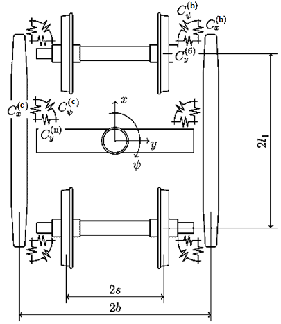
Fig. 1. 3 – piece bogie

We consider the motion only in the horizontal plane. The system consists of (half) the body with a bolster, two side frames and two wheel sets. The body and the bolster are connected by a hinge in the center plate arrangement, the bolster with side frames and the side frames with wheel sets – by elastic elements that prevent relative translational movements in the longitudinal and transverse directions, as well as relative angular movements of hunting of the interacting bodies.

There are no dissipative elements in the system. The degrees of freedom are listed in Table 1. x, y, indicate small movements of recoiling, swaying and hunting, for wheel sets the coordinate is chosen so that  is a small deviation of the angular velocity of wheel set rotation relative to its axis from the value (V is the car velocity, r is the wheel radius), corresponding to the undisturbed motion.

Table 1

Degrees of freedom and generalized coordinates

Body	Degrees of freedom	Generalized coordinates
Body with bolster	, ,	, ,
Left side frame ()	, ,	, ,
Right side frame ()	, ,	, ,
First wheel set ()	, , ,	, …,
Second wheel set ()	, , ,	, …,

We will be interested in how the frequencies and forms of oscillations of the system without constraints (SF) and systems, whose displacement is subject to the following restrictions, correlate:

SCX – it is prohibited to move the bolster relative to the side frames (in the spring suspension openings) in the longitudinal direction;

SAJ – it is prohibited to move the pedestal openings of the side frames relative to the wheel set axle journals (side frames are pivotally connected to the wheel sets).

As for system parameters, the meaning of the notation for rigidity coefficients and basic dimensions is clear from Figure 1: the letters m, I with corresponding indices denote the masses and central moments of body inertia, the coefficients in the expressions for the interaction forces are explained below, the capital letters X, Y, denote the force components and the system body interaction force moments. Without giving a complete derivation of the expressions for the matrices M, L, etc, let us dwell only on certain points that may be of methodical interest. The elements of the matrix C are coefficients for the products of generalized coordinates and their variations in the expression for the virtual work of forces in elastic elements

. (6)

Let us consider the contribution to the matrix C from the elastic elements that are in axle boxes. The components of the displacement of the side frame pedestal opening relative to the wheel set axle box are combined into a vector

.

They are linear combinations of the generalized coordinates

,

,

,

This means that it is possible to choose such matrices with constant coefficients that

.

The force components in the elastic element are proportional to the vector , ,

The virtual work of the forces is equal to

. (7)

Comparing the expressions (6) and (7), we get:

(contributions from other elastic elements).

In order to prohibit linear movements of the pedestal openings of the side frames relative to wheel set axle boxes, it is necessary to require the fulfillment of the conditions:

, .

There are 8 rows in the L matrix, which we get by writing the first two rows of each matrix under each other. Thus, the compilation of a system of equations describing the motion of a mechanical system with constraints does not practically require additional calculations – in our case, the matrices were written out at the stage of working with the system without constraints.

The wheel-rail interaction is described by Kalker linear theory [16 par. 2.2.2] with the following simplifications:

1) spin is neglected;

2) the coefficients , for the longitudinal and transverse directions are considered equal to 3.90.

The expression for longitudinal sliding additionally contains terms proportional to the velocities , .

,

The expression for transverse sliding retains the usual look

.

Findings

Let us consider the results of the calculation of the eigenvalues and eigenvectors describing the 3–piеce bogie oscillations. Our goal is to understand how the eigenvalues and eigenvectors of SF system with constraints and SCX and SAJ systems without constraints are related. We expect that the results for SF with, will tend to the results for SAJ, and the results for SF with – to the results for SCX. The subject of the study will be the confirmation of this expectation and a detailed description of the limiting transition nature.

The eigenvalues of the matrix for the SF and SAJ systems are listed in Table 2. The system parameters correspond to the 4-axle car loaded up to deadweight capacity on 18–100 bogies (with an axle load of 23.5 tf). The motion speed km/h.

The eigenvalues were ordered by the QR algorithm, so they can be compared only by values. Even without analyzing the eigenvectors, it is clear that the numbers with of the SAJ system are the limits for the eigenvalues of the SAF system. It seems plausible to assume that large negative numbers of one system go into large negative numbers of the other system, both systems have five such numbers, but the correspondence between them is not obvious. It is not quite clear which of the numbers of the SF system goes into the number of the SAJ system. The numbers of SF, except for one pair, apparently correspond to the side frame oscillations on the high rigidity elastic elements in the axle boxes, since these numbers have a large imaginary component.

The study of eigenvectors confirms the conclusions made and allows for some refinements. Let us consider the SAJ system with hinges in axle boxes. Equations of constraints do not violate the first 15 eigenvectors:

1, 2) non-physical solutions, which appeared due to the fact that there are no variables in the equations of motion, there are only their derivatives;

3, 4, 13) extremely rapidly decaying solutions describing the motion of wheel sets against pseudo-slip forces (for example, bogie swaying without hunting);

5, 6) bolster hunting oscillations;

7, 8) the same as 3, 4 – rotation of the wheel sets about their axis without longitudinal displacement;

9, 10) body swaying oscillations (wheel sets also have swaying and hunting oscillations, but the ratio of amplitude values and y is less by about 20% than Klingel solution provides);

11, 12) joint oscillations of the wheel set swaying and hunting (amplitude of body oscillations is less than with the forms 9 and 10);

14, 15) bogie oscillations under the body in the longitudinal direction (spring suspension sets are deformed in the longitudinal direction).

Table 2

Eigenvalues for systems SF, SAJ, and SCX

j	, 1/с	j	, 1/с
SF		SAJ
1, 2	0	1, 2	0
3	–1800	3	–990
4	–1640	4	–1140
5, 6	–5610	5, 6	–6.29±335i
7	–1790	7	–5040
8	–1650	8	–3900
9, 10	–56.5±585i	9, 10	–2.33±17.3i
11, 12	–38.2±554i	11, 12	1.24±11.9i
13, 14	–11.9±314i	13	–1440
15, 16	–34.1±874i	14, 15	–0.21±91.1i
17, 18	±857i	16, …, 34	0
19, 20	–3.64±638i	SAJ + SCX
21, 22	±542i	1, 2	0
23, 24	–3.89±315i	3	–4000
25, 26	–2.31±17.1i	4	–3900
27, 28	1.25±11.9i	5	–891
29, 30	–0.21±88.6i	6	–1440
31	–148	7	–1440
32, 33	0	8, 9	–2.33±17.,3i
34	–1.14	10, 11	1.24±11.9i
		12, …, 34	0

For all these vectors, one can find the corresponding eigenvectors of the SF system with close values of the components. Some vectors are shown in Table 3. The vectors , for a bogie without constraints, with large rigidity of elastic elements in the axle boxes are almost coincide with the vectors , for a bogie with hinges in boxes. The vector (SF) describes the longitudinal oscillations of the side frames relative to the wheel sets, which is incompatible with the constraints to which the SAJ system is subordinate, and it is impossible to find a corresponding vector among the eigenvectors of the latter. The bogie movement is unstable, the eigenvalues (SF) and (SAJ) have a positive real part. Wheel sets perform self-oscillations of hunting and swaying (the ratio between the amplitudes y and is as in the Klingel solution), and the body swaying is twice as large as wheel set swaying. Figure 2 shows how the components of the corresponding eigenvector change as rigidity changes

Fig. 2. The principal mode of unstable motion

Table 3

Components of eigenvectors

Compo-	SF						SAJ
nent
					0.67	–1.47			0.67	–1.47
	0.30	1.19	0.98	–1.61	0.13	0.42	1.00	–1.59	0.13	0.40
	0.65	–1.67	0.13	–2.15	0.13	0.42	0.04	2.82	0.14	0.40
	0.06	–2.82			0.34	–1.26			0.34	–1.26
	0.65	1.47	0.13	0.99	0.13	–2.73	0.04	–0.33	0.14	–2.74
	0.06	–2.82			0.34	–1.26			0.34	–1.26
	0.02	1.29			0.33	–1.25			0.34	–1.26

Continuation of the table 3

Compo-	SF						SAJ
nent
	0.16	2.88	0.06	2.80	0.13	0.42	0.04	2.82	0.13	0.40
	0.02	1.29			0.33	–1.25			0.34	–1.26
	0.16	2.88	0.06	2.80	0.13	0.42	0.04	2.82	0.13	0.40

If a rigid longitudinal constraint in the spring suspension is added to the hinges in the axle box (Table 2, column SAJ + SCX), then the oscillation patterns 5, 6, 14, 15 in the SAJ system, which are accompanied by deformations of the spring groups in the longitudinal direction will disappear and four more eigenvectors, corresponding to zero eigenvalues and violating equations of constraints, will be. Other eigenvalues will change slightly.

Originality and practical value

Originality consists in the adaptation of Lyapunov's stability method of linear approximation to the case when the equations of railway vehicle motion are written in the form of differential-algebraic Lagrange equations of the first kind. This written form of the equation of motion makes it possible to simplify the stability study by avoiding the selection of a set of independent generalized coordinates with the subsequent elimination of dependent ones and allows for the coefficient matrix calculation in an easily algorithmized way. Information on the vehicle stability is vitally important, since the truck design must necessarily exclude the loss of stability in the operational speed range.

Conclusions

1. An effective method for studying the stability of railway vehicle motion, described by the Lagrange equations of the first kind, has been proposed. Stability criterion – the real numbers of exponential functions that satisfy the equations of motion – should not be greater than zero. The indicators themselves can be found as eigenvalues of a certain matrix A, depending on the matrices of physical parameters M, B, F, C, K and the matrix of constraint coefficients L, using the QR algorithm [2, chapter 4].

2. The eigenvectors of this matrix, corresponding to nonzero eigenvalues, satisfy the equations of constraints. The advantage of the proposed method is the easy algorithmization of the motion equation derivation (no need to choose independent generalized coordinates).

LIST OF REFERENCE LINKS

1.Деммель, Дж. Вычислительная линейная алгебра. Теория и приложения / Дж. Деммель ; пер. с англ. Х. Д. Икрамова. – Москва : Мир, 2001. – 435 с.

2.Лазарян, В. А. Устойчивость движения рельсовых экипажей / В. А. Лазарян, Л. А. Длугач, М. Л. Коротенко. – Киев : Наук. думка, 1972. – 198 с.

3.Орлова, А. М. Влияние конструктивных схем и параметров тележек на устойчивость, ходовые качества и нагруженность грузовых вагонов : автореф. дис. ... д-ра техн. наук : 05.22.07 / Орлова Анна Михайловна ; Петербург. гос. ун-т путей сообщения. – Санкт-Петербург, 2008. – 32 с.

4.Bigoni, D. Sensitivity analysis of the critical speed in railway vehicle dynamics / D. Bigoni, H. True, A. P. Engsig-Karup // Vehicle System Dynamics. – 2014. – Vol. 54. – Iss. supp1. – P. 272–286.
doi: 10.1080/00423114.2014.898776

5.Critical speed of a Korean high-speed train through optimization with measured wheel profiles / C.-S. Jeon, H.-S. Cho, C.-S. Park, S.-W. Kim, T.-W. Park // Proceedings of the Institution of Mechanical Engineers, Part F: Journal of Rail and Rapid Transit. – 2018. – Vol. 232. – Iss. 1. – P. 171–181.
doi: 10.1177/0954409716662091

6.Gasch, R. Non-linear bogie hunting / R. Gasch, W. Kik, D. Moelle // Vehicle System Dynamics. – 1981. – Vol. 10. – Iss. 2-3. – P. 145–148. doi: 10.1080/00423118108968657

7.Influence of vehicle parameters on critical hunting speed based on Ruzicka model / D. Cui, Li Li, X. Jin,
X. Xiao, J. Ding // Chinese Journal of Mechanical Engineering. – 2012. – Vol. 25. – Iss. 3. –
P. 536–542. doi: 10.3901/cjme.2012.03.536

8.Kalker, J. J. Three-dimensional elastic bodies in rolling contact / J. J. Kalker. – Dordrecht : Springer, 1990. – 314 p. doi: 10.1007/978-94-015-7889-9

9.Mao, X. A design method for rail profiles based on the geometric characteristics of wheel-rail contact /
X. Mao, G. Chen // Proceedings of the Institution of Mechanical Engineers, Part F: Journal of Rail and Rapid Transit. – 2018. – Vol. 232. – Iss. 5. – P. 1255–1265. doi: 10.1177/0954409717720346

10.Mazzola, L. Evaluation of the hunting behavior of a railway vehicle in a curve / L. Mazzola, S. Alfi, S. Bruni // Proceedings of the Institution of Mechanical Engineers, Part F: Journal of Rail and Rapid Transit. – 2014. – Vol. 229. – Iss. 5. – P. 530–541. doi: 10.1177/0954409713517379

11.Moelle, D. Computation of Limit Cycles of a Wheelset Using a Galerkin Method / D. Moelle, H. Steinborn,
R. Gasch // Vehicle System Dynamics. – 1979. – Vol. 8. – Iss. 2-3. – P. 168–171.
doi: 10.1080/00423117908968592

12.Molatefi, H. Critical speed and limit cycles in the empty Y25-freight wagon / H. Molatefi, M. Hecht,
M. H. Kadivar // Proceedings of the Institution of Mechanical Engineers, Part F: Journal of Rail and Rapid Transit. – 2006. – Vol. 220. – Iss. 4. – P. 347–359. doi: 10.1243/09544097jrrt67

13.Polach, O. Bogie design for better dynamic performance: example of a locomotive bogie / O. Polach // European Railway Review. – 2003. – No. 1. – P. 69–77.

14.Polach, O. Comparison of Methods Analyzing Bifurcation and Hunting of Complex Rail Vehicle Models /
O. Polach, I. Kaiser // Journal of Computational and Nonlinear Dynamics. – 2012. – Vol. 7. – Iss. 4.
doi: 10.1115/1.4006825

15.Polach, O. Compatibility of the non-linear and linearized stability assessment during railway vehicle design / O. Polach // Vehicle System Dynamics. – 2006. – Vol. 44. – Iss. sup1. – P. 129–138.
doi: 10.1080/00423110600869537

16.True, H. The Dynamics of a Railway Freight Wagon Wheelset with Dry Friction Damping / H. True, R. Asmund // Vehicle System Dynamics. – 2002. – Vol. 38. – Iss. 2. – P. 149–163. doi: 10.1076/vesd.38.2.149.5617

17.Xia, F. On the dynamics of the three-piece-freight truck / F. Xia, H. True // Proceedings of the 2003 IEEE/ASME Joint Rail Conference. – 2003. – P. 149–159. doi: 10.1109/rrcon.2003.1204661

О. Г. РЕЙДЕМЕЙСТЕР^1*, С. І. Левицька^2*

^1*Каф. «Вагони та вагонне господарство», Дніпропетровський національний університет залізничного
транспорту імені академіка В. Лазаряна, вул. Лазаряна, 2, Дніпро, Україна, 49010, тел. +38 (056) 373 15 19,
ел. пошта reidemeister.a@gmail.com, ORCID 0000-0001-7490-7180
^2*Каф. «Іноземні мови», Придніпровська державна академія будівництва та архітектури,
вул. Чернишевського, 24А, Дніпро, Україна, 49000, тел. +38 (056) 756 33 56,
ел. пошта svetik23com@ukr.net, ORCID 0000-0001-6725-0280

Стійкість руху залізничних екіпажів,

ЯКИЙ описують рівняння Лагранжа I роду

Мета. У статті необхідно оцінити стійкість руху залізничних екіпажів, коливання яких описані рівняннями Лагранжа I роду, в припущенні, що відсутні нелінійності з розривами правих частин. Методика. За основу прийнято метод дослідження стійкості руху Ляпунова за лінійним наближенням. Рівняння руху складено в матричній формі. Сили кріпа обчислені у відповідності з лінійної теорією Калкера. Послідовними диференціюваннями рівнянь зв’язків індекс системи рівнянь знижений з 2 до 0. Власні числа матриці коефіцієнтів отриманої таким чином системи знайдені за допомогою QR-алгоритму. Відповідно до критерію Ляпунова про стійкість за лінійним наближенням рух стійкий, якщо у всіх власних чисел дійсна частина негативна. Нетривіальним є наявність «зайвих» ступенів свободи, яких немає у механічної системи (в її рівняннях руху залишили тільки незалежні координати). Цим ступеням свободи відповідають власні числа і власні вектори, що не мають відношення до стійкості. Щоб знайти правило, що дозволяє їх виключити, ми розглянули кілька моделей візків, із жорсткими і пружними зв’язками великої жорсткості у вузлах. У граничному випадку великих жорсткостей результати для системи без жорстких зв’язків повинні співпасти з результатами для системи з жорсткими зв’язками. Результати. Проведено аналіз і зіставлені частоти (з декрементом) і форми коливань 3-елементного візка зі зв’язками і без них. При аналізі стійкості системи зі зв’язками становлять інтерес тільки ті власні числа, власні вектори яких не порушують зв’язків. Значення цих чисел є межами для власних чисел системи, в якій жорсткі зв’язки замінені пружними елементами великої жорсткості, що дозволяє залишити критерій Ляпунова незмінним. Наукова новизна полягає в адаптації методу дослідження стійкості руху Ляпунова за лінійним наближенням до випадку, коли рівняння руху залізничних екіпажів записані в формі диференційно-алгебраїчних рівнянь Лагранжа I роду. Практична значимість. Зазначена форма запису рівняння руху дозволяє спростити дослідження стійкості за рахунок відмови від виділення безлічі незалежних узагальнених координат із наступним виключенням залежних і допускає обчислення матриці коефіцієнтів легко алгоритмізованим способом. Інформація про стійкість екіпажів украй важлива, оскільки конструкція ходових частин повинна в обов’язковому порядку виключати втрату стійкості в експлуатаційному діапазоні швидкостей.

Ключові слова: залізничний екіпаж; стійкість руху; диференційно-алгебраїчні рівняння

А. Г. РЕЙДЕМЕЙСТЕР^1*, С. И. ЛЕВИЦКАЯ^2*

^1*Каф. «Вагоны и вагонное хозяйство», Днепропетровский национальный университет железнодорожного
транспорта имени академика В. Лазаряна, ул. Лазаряна, 2, Днипро, Украина, 49010, тел. +38 (056) 373 15 19,
эл. почта reidemeister.a@gmail.com, ORCID 0000-0001-7490-7180

^2*Каф. «Иностранные языки», Приднепровская государственная академия строительства и архитектуры,
ул. Чернышевского, 24А, Днипро, Украина, 49000, тел. +38 (056) 756 33 56,
эл. почта svetik23com@ukr.net, ORCID 0000-0001-6725-0280


УСТОЙЧИВОСТЬ ДВИЖЕНИЯ ЖЕЛЕЗНОДОРОЖНЫХ

ЭКИПАЖЕЙ, ОПИСЫВАЕМого УРАВНЕНИЯМИ

ЛАГРАНЖА I РОДА

Цель. В статье необходимо оценить устойчивость движения железнодорожных экипажей, колебания которых описаны уравнениями Лагранжа I рода, в предположении, что отсутствуют нелинейности с разрывами правых частей. Методика. За основу принят метод исследования устойчивости движения Ляпунова по линейному приближению. Уравнения движения составлены в матричной форме. Силы крипа вычислены в соответствии с линейной теорией Калкера. Последовательными дифференцированиями уравнений связей индекс системы уравнений понижен с 2 до 0. Собственные числа матрицы коэффициентов полученной таким образом системы найдены с помощью QR–алгоритма. В соответствии с критерием Ляпунова об устойчивости по линейному приближению движение устойчиво, если у всех собственных чисел действительная часть отрицательна. Нетривиальным является наличие «лишних» степеней свободы, которых нет у механической системы (в ее уравнениях движения оставили только независимые координаты). Этим степеням свободы соответствуют собственные числа и собственные векторы, к устойчивости отношения не имеющие. Чтобы найти правило, позволяющее их исключить, мы рассмотрели несколько моделей тележки, с жесткими и упругими связями большой жесткости в узлах. В предельном случае больших жесткостей результаты для системы без жестких связей должны совпасть с результатами для системы с жесткими связями.
Результаты. Проведен анализ и сопоставлены частоты (с декрементами) и формы колебаний 3–элементной тележки со связями и без них. При анализе устойчивости системы со связями представляют интерес только те собственные числа, собственные векторы которых не нарушают связей. Значения этих чисел являются пределами для собственных чисел системы, в которой жесткие связи заменены упругими элементами большой жесткости, что позволяет оставить критерий Ляпунова неизменным. Научная новизна состоит в адаптации метода исследования устойчивости движения Ляпунова по линейному приближению к случаю, когда уравнения движения железнодорожных экипажей записаны в форме дифференциально-алгебраических уравнений Лагранжа I рода. Практическая значимость. Указанная форма записи уравнения движения позволяет упростить исследование устойчивости за счет отказа от выделения множества независимых обобщенных координат с последующим исключением зависимых и допускает вычисление матрицы коэффициентов легко алгоритмизируемым способом. Информация об устойчивости экипажей крайне важна, поскольку конструкция ходовых частей должна в обязательном порядке исключать потерю устойчивости в эксплуатационном диапазоне скоростей.

Ключевые слова: железнодорожный экипаж; устойчивость движения; дифференциально-алгебраические уравнения